Google App Script 之 SpreadsheetApp
Google App Script 中的 SpreadsheetApp 服务可以读取、创建、修改 Google Sheet。
例如下方代码,SpreadsheetApp.getActiveSpreadsheet()方法得到当前表格文件对象(Spreadsheet),currentSpreadsheet.getActiveSheet()方法得到当前工作表对象(Sheet),currentSheet.getCurrentCell()得到当前活动单元格对象(Range),再通过单元格对象的getValue方法获取到活动单元格的值。
function logCurrent() {
  let currentSpreadsheet = SpreadsheetApp.getActiveSpreadsheet()
  let currentSheet = currentSpreadsheet.getActiveSheet();
  let currentRange = currentSheet.getCurrentCell();
  console.log(currentRange.getValue());
}
由小到大,可以把 Google Sheet 分为 Range、RangeList、Sheet、Spreadsheet。
Range
Range 是 Google Sheet 里的最小元素,表示单元格的区域,可以是一个单元格或者是一组单元格。
当是一个单元格时可以用getValue()方法获取单元格显示的值,返回字符串;当是一组单元格则需要用getValues()来获取值,返回一个二维数组,第一层为行,第二层为列。
如下图,data最终的值为[[1,2],[3,4]]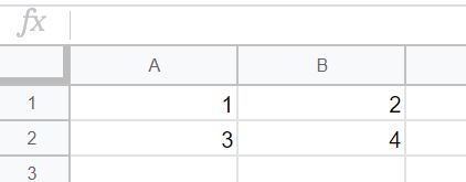
function logData() {
  let sheet = SpreadsheetApp.getActiveSheet();
  let range = sheet.getDataRange()
  let data = range.getValues();
  console.log(data);
}